Fully Connected Layers & CNN Training: The Voting System!

ফুল্লি কানেক্টেড লেয়ার ও ট্রেনিং: ভোট গ্রহণ এবং ভুল সংশোধন!

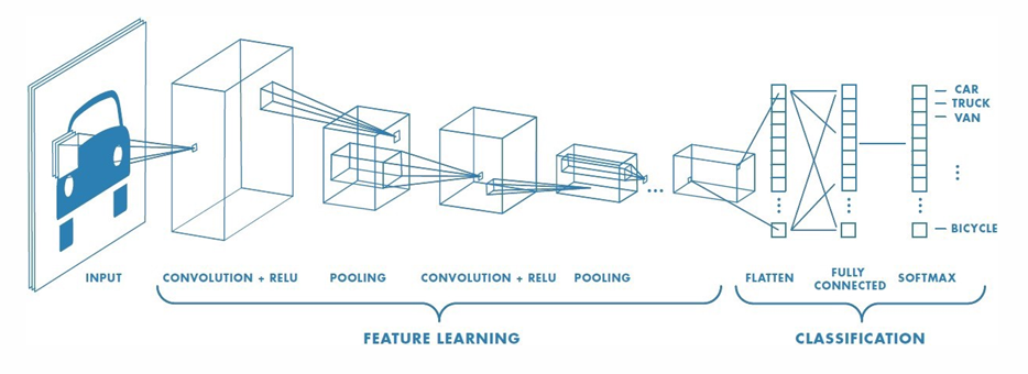
Hello! Now that we know how a CNN extracts features from an image using Convolutions and Pooling, we arrive at the big question: How does it actually make the final decision? How does it confidently say, "Yes, that is a CAR!"?

This happens in the second half of the CNN architecture!

The Two Halves of a CNN

A complete CNN model is always split into two distinct parts:

1. Feature Learning (The Eyes): The Convolutional and Pooling layers that extract all the best features (edges, wheels, shapes).
2. Classification (The Brain): The Fully Connected (FC) Layer that takes those features and makes the final decision.

Before passing the data from the eyes to the brain, we have to Flatten it. This simply means taking all the 2D feature maps and stretching them out into one single, incredibly long 1D line of numbers (a vector).

Fully Connected Layer (The Voting System)

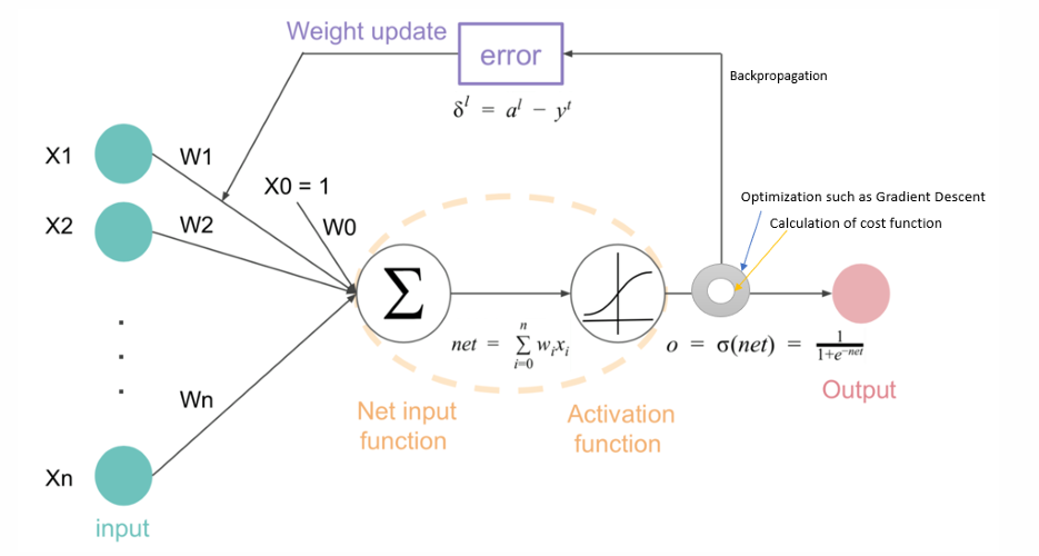
The FC layer is essentially a MultiLayer Perceptron (MLP). It contains an Input layer, Hidden layer(s), and an Output layer. Every single neuron in this layer has inputs ($x$), weights ($w$), and a bias ($b$). The mathematical formula is the classic Perceptron equation: $$output = \text{ActivationFunction}(x_0 \cdot w_0 + x_1 \cdot w_1 + \dots + x_n \cdot w_n + \text{bias})$$

Real-life Analogy: Think of the FC layer as a massive democratic voting system. Every extracted feature (like "fur", "pointy ears", "whiskers") casts a vote. The weights are how much we trust each vote. If the "whiskers" feature is highly activated, it casts a heavy vote for the "CAT" category. The category with the most votes wins!

Activation Functions (The Final Filter)

To convert these mathematical votes into a format we can understand, we use Activation Functions at the very end:

• Sigmoid: Outputs a smooth curve between 0 and 1. (Great for binary questions: "Is it a cat or a dog?").
• Softmax: Used for multi-class problems. It turns the final votes into a clean probability distribution that adds up to 100%. (e.g., 80% Cat, 15% Dog, 5% Mouse).
• Tanh: Similar to Sigmoid but outputs between -1 and +1.
• Hardlim: A strict step function. If the number is below 0, output is 0. If it's above 0, output is 1. No smooth transitions!

Training: How does the CNN Learn? (Back-propagation)

Initially, the CNN is completely dumb because all its weights (the voting power) are random! To teach it, we use a dataset with images and correct labels, and apply an algorithm called Back-propagation.

1. Make a Guess: We show it an image of a cat. The untrained model guesses "Dog".
2. Calculate the Error: We say, "Wrong! The answer is Cat." The mathematical difference between its guess and the real answer is the Error.
3. Back-propagation: The model takes this error and sends it backwards through the entire network, from the output layer all the way to the first convolution layer.
4. Update Weights: It slightly adjusts all the weights using Gradient Descent so that next time, it is more likely to guess "Cat".

Real-life Analogy: It is exactly like checking an exam paper. You see how wrong the final answer is (Error), then you trace back through the student's math to find exactly which step caused the mistake, and correct it so they don't do it again!

[!NOTE] IMPORTANT NOTES FOR NOTEBOOK Concept: Fully Connected Layers & Back-propagation Key Point 1: A CNN is split into feature learning (Conv/Pool) and classification (Fully Connected). Key Point 2: The FC layer acts as a weighted voting system: $output = \text{ActivationFunction}(\sum(x_i \cdot w_i) + \text{bias})$. Key Point 3: Softmax is heavily used in the output layer to provide a normalized probability distribution across multiple classes. Key Point 4: Back-propagation calculates the error at the output and propagates it backwards to iteratively update the network's weights via Gradient Descent.

হ্যালো! গত পর্বে আমরা দেখেছি CNN কীভাবে কনভোল্যুশন এবং পুলিং ব্যবহার করে ছবি থেকে ফিচার বা বৈশিষ্ট্য বের করে আনে। আজ আমরা সবচেয়ে বড় প্রশ্নের উত্তর খুঁজবো: CNN আসলে তার চূড়ান্ত সিদ্ধান্তটি কীভাবে নেয়? কীভাবে সে এত আত্মবিশ্বাসের সাথে বলে, "হ্যাঁ, এটি একটি গাড়ি!"?

এই জাদুকরী কাজটি ঘটে CNN আর্কিটেকচারের দ্বিতীয় অংশে!

CNN-এর দুটি অংশ

একটি সম্পূর্ণ CNN মডেলকে সাধারণত দুটি প্রধান অংশে ভাগ করা যায়: ১. Feature Learning (চোখ): কনভোল্যুশনাল এবং পুলিং লেয়ার, যারা ছবির সেরা ফিচারগুলো (যেমন- চাকা, আকৃতি, রেখা) বের করে আনে। ২. Classification (মস্তিষ্ক): Fully Connected (FC) Layer, যা সেই ফিচারগুলো নিয়ে চূড়ান্ত সিদ্ধান্ত গ্রহণ করে।

চোখ থেকে মস্তিষ্কে ডেটা পাঠানোর আগে আমাদের ডেটাকে Flatten করতে হয়। এর মানে হলো, 2D বা দ্বিমাত্রিক ফিচার ম্যাপগুলোকে টেনে লম্বা করে এক লাইনের একটি বিশাল 1D ভেক্টরে রূপান্তর করা।

ফুল্লি কানেক্টেড লেয়ার (ভোট গ্রহণ সিস্টেম)

FC লেয়ারটি মূলত একটি MultiLayer Perceptron (MLP)। এর মধ্যে একটি ইনপুট লেয়ার, হিডেন লেয়ার এবং একটি আউটপুট লেয়ার থাকে। এই লেয়ারের প্রতিটি নিউরনে ইনপুট ($x$), ওয়েট ($w$) এবং বায়াস ($b$) থাকে। এর গাণিতিক সমীকরণটি হলো আমাদের চিরচেনা পারসেপট্রন ইকুয়েশন: $$output = \text{ActivationFunction}(x_0 \cdot w_0 + x_1 \cdot w_1 + \dots + x_n \cdot w_n + \text{bias})$$

বাস্তব জীবনের উদাহরণ: তুমি FC লেয়ারকে একটি বিশাল গণতান্ত্রিক ভোটিং সিস্টেম হিসেবে ভাবতে পারো! প্রতিটি ফিচার (যেমন- "লোম", "চোখা কান", "গোঁফ") হলো এক একজন ভোটার। আর ওয়েট (weight) হলো আমরা কার ভোটকে কতটা গুরুত্ব দিচ্ছি। যদি ছবিতে "গোঁফ" ফিচারটি খুব বেশি দেখা যায়, তবে সেটি "বিড়াল" ক্যাটাগরিতে একটি বিশাল ভোট দেয়। দিনশেষে যে ক্যাটাগরি সবচেয়ে বেশি ভোট পায়, সে-ই জয়ী হয়!

অ্যাক্টিভেশন ফাংশন (ফাইনাল ফিল্টার)

এই গাণিতিক ভোটগুলোকে আমাদের বোঝার মতো ফর্মে রূপান্তর করতে লেয়ারের একদম শেষে কিছু অ্যাক্টিভেশন ফাংশন ব্যবহার করা হয়:

• Sigmoid: এটি ০ থেকে ১ এর মধ্যে একটি মসৃণ (S-আকৃতির) মান দেয়। (হ্যাঁ/না জাতীয় প্রশ্নের জন্য দারুণ কাজ করে)।
• Softmax: মাল্টি-ক্লাস সমস্যার জন্য এটি সবচেয়ে জনপ্রিয়। এটি ফাইনাল ভোটগুলোকে একটি পারফেক্ট Probability distribution-এ রূপান্তর করে, যার যোগফল হয় ১০০%। (যেমন- ৮০% বিড়াল, ১৫% কুকুর, ৫% ইঁদুর)।
• Tanh: সিগময়ডের মতোই, তবে এর মান -১ থেকে +১ এর মধ্যে থাকে।
• Hardlim: এটি একটি কড়া স্টেপ ফাংশন। মান ০-এর কম হলে আউটপুট ০, আর ০ বা তার বেশি হলে আউটপুট ১। এখানে মাঝামাঝি কোনো মান নেই!

ট্রেনিং: CNN কীভাবে শেখে? (Back-propagation)

শুরুতে একটি CNN একদম বোকা থাকে, কারণ তার সমস্ত ওয়েট (ভোটের ক্ষমতা) রেন্ডম বা এলোমেলোভাবে দেওয়া থাকে! তাকে শেখানোর জন্য আমরা অনেক ছবি ও সঠিক লেবেল (উত্তর)-সহ একটি ডেটাসেট নিই এবং Back-propagation (ব্যাক-প্রোপাগেশন) নামক অ্যালগরিদম ব্যবহার করি।

১. অনুমান করা: আমরা তাকে একটি বিড়ালের ছবি দেখালাম। আনট্রেইনড মডেলটি আন্দাজে বললো "কুকুর"। ২. ভুল হিসাব করা (Error): আমরা বললাম, "ভুল! সঠিক উত্তর হলো বিড়াল।" তার অনুমান এবং সঠিক উত্তরের মাঝের গাণিতিক পার্থক্যটিই হলো Error বা ভুল। ৩. ব্যাক-প্রোপাগেশন: মডেলটি এই ভুলের পরিমাণটা নেয় এবং নেটওয়ার্কের একদম আউটপুট থেকে পেছনের দিকে প্রথম লেয়ার পর্যন্ত পাঠাতে থাকে। ৪. ওয়েট আপডেট: সে Gradient Descent ব্যবহার করে তার সব ওয়েট একটু একটু করে পরিবর্তন করে বা শুধরে নেয়, যাতে পরের বার সে ঠিকমতো "বিড়াল" বলতে পারে!

বাস্তব জীবনের উদাহরণ: এটি ঠিক পরীক্ষার খাতা দেখার মতো! তুমি প্রথমে দেখো চূড়ান্ত উত্তরটা কতটা ভুল হয়েছে (Error), এরপর তুমি খাতার পেছন দিকে গিয়ে খোঁজার চেষ্টা করো ঠিক কোন লাইনে ছাত্রটি ভুল করেছিল। তারপর তুমি সেই ভুলটা ধরিয়ে দাও বা সংশোধন করে দাও, যাতে সে পরবর্তীতে আর একই ভুল না করে!

[!NOTE] IMPORTANT NOTES FOR NOTEBOOK Concept: Fully Connected Layers & Back-propagation Key Point 1: A CNN is split into feature learning (Conv/Pool) and classification (Fully Connected). Key Point 2: The FC layer acts as a weighted voting system: $output = \text{ActivationFunction}(\sum(x_i \cdot w_i) + \text{bias})$. Key Point 3: Softmax is heavily used in the output layer to provide a normalized probability distribution across multiple classes. Key Point 4: Back-propagation calculates the error at the output and propagates it backwards to iteratively update the network's weights via Gradient Descent.