Function Composition & The Universal Approximation Theorem
ফাংশন কম্পোজিশন ও ইউনিভার্সাল অ্যাপ্রোক্সিমেশন থিওরেম!
Hello! This is our grand finale on the Deep Learning Basics series! Today, we will look at neural networks from a pure mathematical perspective, visualize what they actually 'see', and discover just how incredibly powerful they truly are!
Function Composition: The Math of Layers (A Game of Telephone)
Did you know that every layer in a neural network is just calculating a mathematical function? Therefore, the entire network is simply a massive chain or composition of functions! Think of it like the game of Telephone, but instead of words getting messed up, they get refined. $h^{(1)} = f^{(1)}(x)$ (Person A tells Person B) $h^{(2)} = f^{(2)}(h^{(1)})$ (Person B tells Person C) $\dots$ $y = f^{(L)}(h^{(L-1)})$ (The final person shouts the answer)
In short: $y = f^{(L)} \circ \dots \circ f^{(1)}(x)$. This system is highly Modular. It means we can treat every single layer as an independent "black box". Because they are modular, it is super easy to snap them together like Lego bricks and stack hundreds of layers!
Visualizing Feature Learning (The Detective Work)
Let's see this in action using the famous MNIST dataset (handwritten digits). An input image of a digit is a long vector of 784 pixels (28x28).
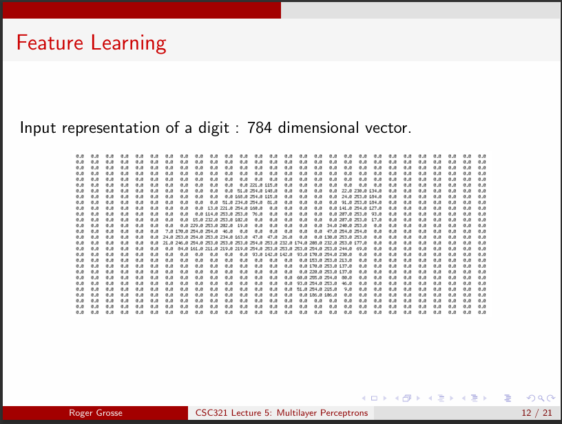
When the network starts learning, what does the first hidden layer actually look for? Imagine the network is a blindfolded detective trying to identify an object by touching it. First, they feel the edges. Then, they feel the curves. Finally, they realize it's a cup! If we convert the mathematical weights of the hidden units into images, we can literally see what the AI detective is learning!
Look at this Feature Bank showing 256 first-level features:
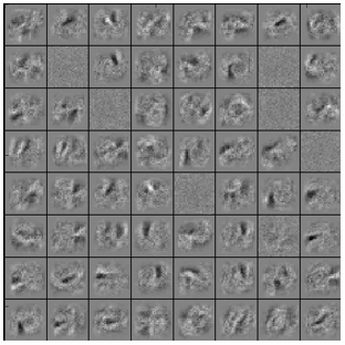
In these tiny boxes, gray means 0, white means positive weight, and black means negative weight. The network has automatically taught itself to detect specific curves, straight lines, strokes, and edges! No human told it what an "edge" was. It built its own edge detectors from scratch just by looking at the pixels!
Levels of Abstraction (Zooming In and Out)
When designing these networks, we must think like the famous computer scientist Don Knuth suggested—we must jump between different levels of abstraction. Think of Google Earth: zooming all the way out to see the globe, and zooming all the way in to see a single house.
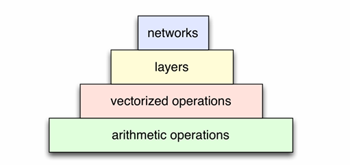
- Networks: The macro view (the overall global architecture).
- Layers: The specific functions of each layer (the countries).
- Vectorized operations: Matrix multiplications (the cities).
- Arithmetic operations: Basic addition/subtraction at the core (the individual houses).
Expressive Power & The Universal Approximation Theorem (The Magic Wand)
Finally, how powerful are these networks? First, a warning: If you stack many linear layers without non-linear activation functions, your deep network is mathematically equivalent to a single, simple linear regression. It becomes incredibly weak!
But, if you add just one hidden layer and use a Nonlinear activation function (like Sigmoid or ReLU), something magical happens. According to the Universal Approximation Theorem:
A feed-forward neural network with at least one hidden layer and a non-linear activation function can perfectly approximate any continuous mathematical function to any desired degree of accuracy!
Yes, it becomes a Universal Approximator! It is literally a mathematical magic wand. If there is a hidden pattern connecting A to B in the universe, this neural network can find it. For binary inputs, you might need a hidden layer with $2^D$ nodes (which is insanely wide), but the mathematical truth remains—neural networks have virtually limitless expressive power!
[!NOTE] IMPORTANT NOTES FOR NOTEBOOK Concept: Function Composition & Universal Approximation Key Point 1: Deep networks function mathematically as a modular chain of composite functions: $y = f^{(L)} \circ \dots \circ f^{(1)}(x)$. Key Point 2: The Universal Approximation Theorem states that a neural network with just one hidden layer and non-linear activations can approximate any continuous function. Advantage: Visualizing weight matrices proves that networks independently extract meaningful geometric shapes from raw pixels. The theoretical power of networks is virtually limitless. Disadvantage: While a single hidden layer can approximate anything, it might need an exponentially wide number of neurons, making deep (multi-layered) networks much more practical and efficient than extremely wide, shallow ones.
হ্যালো! আজ আমাদের ডিপ লার্নিং বেসিকস সিরিজের গ্র্যান্ড ফিনালে বা শেষ পর্ব! আজ আমরা নিউরাল নেটওয়ার্ককে গাণিতিক দৃষ্টিকোণ থেকে দেখবো, ভিজ্যুয়ালাইজ করবো যে এরা আসলে কী 'দেখে', এবং জানবো এদের সত্যিকারের ক্ষমতা কতটা জাদুকরী!
ফাংশন কম্পোজিশন (গাণিতিক চেইন)
তুমি কি জানো, নিউরাল নেটওয়ার্কের প্রতিটি লেয়ার আসলে এক একটি গাণিতিক ফাংশন হিসাব করে? তাই পুরো নেটওয়ার্কটিকে অনেকগুলো ফাংশনের সমষ্টি বা চেইন হিসেবে দেখা যায়! এটা অনেকটা আমাদের ছোটবেলার 'কানে কানে কথা বলা' বা 'টেলিফোন' গেমের মতো। তবে এখানে তথ্য নষ্ট না হয়ে আরও পরিশুদ্ধ হয়! $h^{(1)} = f^{(1)}(x)$ (১ম জন ২য় জনকে বললো) $h^{(2)} = f^{(2)}(h^{(1)})$ (২য় জন ৩য় জনকে বললো) $\dots$ $y = f^{(L)}(h^{(L-1)})$ (শেষ জন উত্তরটা চিৎকার করে বলে দিলো!)
সহজ কথায়, $y = f^{(L)} \circ \dots \circ f^{(1)}(x)$। এই সিস্টেমটি অত্যন্ত Modular (মডুলার)। এর অর্থ হলো, আমরা প্রতিটি লেয়ারের গণনাকে একটি স্বাধীন "ব্ল্যাক বক্স" হিসেবে বিবেচনা করতে পারি। লেগোর (Lego) ব্লকগুলো যেমন একটার ওপর একটা বসিয়ে বিশাল বিল্ডিং বানানো যায়, মডুলার হওয়ার কারণে লেয়ারগুলোকেও আমরা সেভাবেই একটার ওপর একটা বসাতে পারি!
ফিচার লার্নিংয়ের ভিজ্যুয়ালাইজেশন (গোয়েন্দার কাজ)
চলো বিখ্যাত MNIST ডেটাসেট (হাতে লেখা ডিজিট) দিয়ে এর একটি বাস্তব উদাহরণ দেখি। একটি অঙ্কের ছবির ইনপুট হলো ৭৮৪ মাত্রার একটি বিশাল ভেক্টর (২৮x২৮ পিক্সেল)।
নেটওয়ার্ক যখন শিখতে শুরু করে, তখন তার প্রথম হিডেন লেয়ারটি আসলে কী খোঁজে? ধরো নেটওয়ার্কটি একজন চোখ-বাঁধা গোয়েন্দা। সে হাত দিয়ে ছুঁয়ে ছুঁয়ে বুঝতে চাইছে জিনিসটা কী। প্রথমে সে জিনিসের ধার বা প্রান্ত (edge) অনুভব করে, তারপর বাঁক (curve) অনুভব করে, তারপর সে বুঝতে পারে, "ওহ! এটা তো একটা মগ!"
আমরা যদি হিডেন ইউনিটের গাণিতিক ওয়েটগুলোকে (weights) ছবিতে রূপান্তর করি, তবে আমাদের AI গোয়েন্দাটি ঠিক কী শিখছে তা আমরা আক্ষরিক অর্থেই চোখে দেখতে পাবো!
নিচের ২৫৬টি ফার্স্ট-লেভেল ফিচারের এই বিশাল গ্রিড বা ফিচার ব্যাংকটি দেখো:
এই ছোট ছোট বক্সগুলোর মধ্যে ধূসর রঙের মানে ০, সাদার মানে পজিটিভ (+) ওয়েট এবং কালোর মানে নেগেটিভ (-) ওয়েট। অবাক করার মতো বিষয় হলো, কোনো মানুষ তাকে বলে দেয়নি যে "দাগ" বা "বাঁক" কাকে বলে। সে পিক্সেলগুলো দেখে নিজে থেকেই ডিজিটের বিভিন্ন স্ট্রোক, বাঁক বা রেখা সনাক্ত করতে শিখে গেছে!
অ্যাবস্ট্রাকশনের লেভেল (জুম-ইন এবং জুম-আউট)
বিখ্যাত কম্পিউটার বিজ্ঞানী ডন নুথ বলেছিলেন, একজন প্রোগ্রামারের আসল দক্ষতা হলো খুব দ্রুত অ্যাবস্ট্রাকশনের বিভিন্ন লেভেলের মধ্যে পরিবর্তন করতে পারা। অনেকটা গুগল আর্থের মতো—পুরো পৃথিবী দেখা থেকে জুম করে একদম নিজের বাড়ির ছাদে চলে আসা!
১. Networks (নেটওয়ার্ক): পুরো আর্কিটেকচারের ম্যাক্রো ভিউ (পুরো পৃথিবী)। ২. Layers (লেয়ারসমূহ): প্রতিটি নির্দিষ্ট স্তর (দেশসমূহ)। ৩. Vectorized operations: ম্যাট্রিক্সের গুণন (শহরসমূহ)। ৪. Arithmetic operations: একদম মূলে থাকা যোগ-বিয়োগের সাধারণ হিসাব (বাড়িঘর)।
প্রকাশ ক্ষমতা ও ইউনিভার্সাল অ্যাপ্রোক্সিমেশন থিওরেম (জাদুর কাঠি!)
সবশেষে, এই নেটওয়ার্কগুলো ঠিক কতটা শক্তিশালী? প্রথমেই একটি সতর্কতা: তুমি যদি কোনো নন-লিনিয়ার অ্যাক্টিভেশন ফাংশন ছাড়া পরপর অনেকগুলো লিনিয়ার লেয়ার যুক্ত করো, তবে গাণিতিকভাবে তোমার মডেলটি সাধারণ একটি লিনিয়ার রিগ্রেশনের মতোই দুর্বল হয়ে যাবে!
কিন্তু, তুমি যদি শুধু একটিমাত্র হিডেন লেয়ার যোগ করো এবং সেখানে Nonlinear activation function (যেমন Sigmoid বা ReLU) ব্যবহার করো, তবে ম্যাজিক শুরু হবে। Universal Approximation Theorem বা সার্বজনীন অনুমান উপপাদ্য অনুযায়ী:
একটি ফিড-ফরওয়ার্ড নিউরাল নেটওয়ার্কে অন্তত একটি হিডেন লেয়ার এবং নন-লিনিয়ার অ্যাক্টিভেশন থাকলে, সেটি পৃথিবীর যেকোনো কন্টিনিউয়াস (নিরবচ্ছিন্ন) গাণিতিক ফাংশনকে যেকোনো মাত্রায় নিখুঁতভাবে সমাধান বা অনুমান করতে পারে!
হ্যাঁ, এটি একটি Universal Approximator হয়ে যায়! এটি আক্ষরিক অর্থেই একটি গাণিতিক জাদুর কাঠি। যদি মহাবিশ্বে A থেকে B-এর মধ্যে কোনো গাণিতিক সম্পর্ক থাকে, তবে একটি নিউরাল নেটওয়ার্ক তা ঠিকই খুঁজে বের করতে পারবে! যদিও বাইনারি ইনপুটের ক্ষেত্রে একটি মাত্র লেয়ার দিয়ে এই কাজ করতে লেয়ারটিকে প্রচুর চওড়া ($2^D$ নোড) হতে হবে, কিন্তু তাত্ত্বিকভাবে এটি প্রমাণিত যে নিউরাল নেটওয়ার্কের ক্ষমতা সীমাহীন!
[!NOTE] IMPORTANT NOTES FOR NOTEBOOK Concept: Function Composition & Universal Approximation Key Point 1: Deep networks function mathematically as a modular chain of composite functions: $y = f^{(L)} \circ \dots \circ f^{(1)}(x)$. Key Point 2: The Universal Approximation Theorem states that a neural network with just one hidden layer and non-linear activations can approximate any continuous function. Advantage: Visualizing weight matrices proves that networks independently extract meaningful geometric shapes from raw pixels. The theoretical power of networks is virtually limitless. Disadvantage: While a single hidden layer can approximate anything, it might need an exponentially wide number of neurons, making deep (multi-layered) networks much more practical and efficient than extremely wide, shallow ones.