Multilayer Perceptrons (MLP) & Conquering the XOR Problem
মাল্টিলেয়ার পারসেপট্রন (MLP) ও XOR প্রবলেম জয়!
Hello once again! Today we are entering the second phase of our learning, focusing on actual network architectures. Let's talk about Multilayer Perceptrons (MLP) and how they effortlessly solve problems that simple linear models cannot!
Network Design Choices
When starting a neural network project, we have to make 4 major decisions. Think of it like planning a road trip:
- Task: Where are we going? Are we predicting a number (Regression) or classifying categories?
- Architecture: What car are we driving? Will it be a simple linear model or a deep feed-forward network?
- Loss function: How do we know if we took a wrong turn? (Squared error for numbers, Cross-entropy for categories).
- Optimization: How do we steer the car back on track? (Usually using Gradient Descent).
Understanding the Graph (DAG) & MLP
When we connect multiple neurons together without any cycles or loops, we form a Directed Acyclic Graph (DAG). This simply means information flows in a one-way street, never looping back. This is the structural foundation of a Feed-forward Neural Network.
Look at this typical layer arrangement:
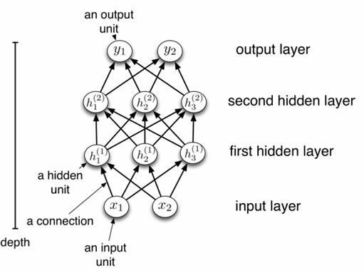 At the bottom, we have the Input Layer. In the middle, the Hidden Layers. At the top, the Output Layer.
If every neuron in one layer connects directly to every single neuron in the next layer, we call it a Fully Connected Layer. A network built entirely with these layers is famously known as a Multilayer Perceptron (MLP)! It's the bread and butter of Deep Learning.
A Closer Look at Activation Functions
Before we solve the famous XOR problem, let's take a quick look at the exact mathematical shapes of the activation functions we use to power our neurons.
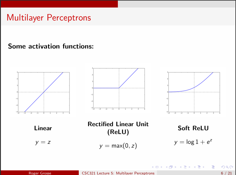
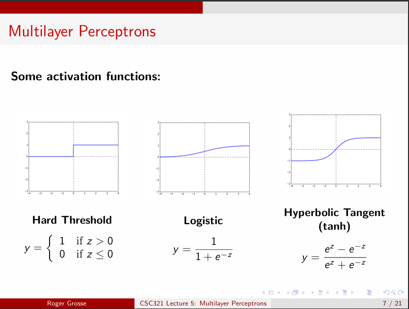 These graphs beautifully illustrate how different functions like Linear, ReLU, Softplus, Hard Threshold, Sigmoid (Logistic), and Tanh behave mathematically!
The Infamous XOR Problem (A Bad Relationship Analogy)
Here is a classic problem in computer science: A simple linear classifier cannot solve the XOR logic gate problem.
Why? Imagine you have two couples sitting at a square table. Couple A is sitting at opposite diagonal corners (the 1s), and Couple B is sitting at the other two diagonal corners (the 0s). They are currently having a huge fight, and you need to separate Couple A from Couple B by drawing a single straight line across the table. Because they are sitting diagonally, it is physically impossible! The data points of XOR are not "linearly separable".
So, how does a neural network solve this relationship drama?
By adding a Hidden Layer (a mediator)!
Look at this 2-layer MLP designed specifically to solve XOR using Hard Threshold activation functions:
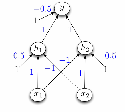
- How the mediator works: We have two inputs ($x_1, x_2$) representing the couples on the table.
- The first hidden node $h_1$ is given weights $[1, -1]$ and a bias of $-0.5$.
- The second hidden node $h_2$ gets weights $[-1, 1]$ and a bias of $-0.5$.
- The final output node $y$ combines them with weights $[1, 1]$ and a bias of $-0.5$.
Why does this matter? By manually setting these specific weights, the hidden layer (the mediator) essentially tells one of the couples to stand up on a chair! Now, with one couple in the air (3D space) and the other still sitting on the table, you can easily slide a flat sheet of cardboard between them to separate them.
This proves mathematically that adding hidden layers vastly expands the power of a model by mapping impossible 2D problems into higher dimensions where they become easily solvable!
[!NOTE] IMPORTANT NOTES FOR NOTEBOOK Concept: Multilayer Perceptron (MLP) & XOR Problem Key Point 1: MLPs are Directed Acyclic Graphs (DAGs) consisting of fully connected layers where information flows in a single forward direction. Key Point 2: Linear models fail at the XOR function because it is not linearly separable. However, introducing a hidden layer maps the inputs into a new space where XOR becomes linearly solvable. Advantage: Concrete proof that adding intermediate layers breaks linear boundaries and vastly broadens the functional capability of AI. Disadvantage: Fully connected layers have a massive number of parameters, making them computationally expensive and prone to overfitting.
হ্যালো! আজ আমরা আমাদের লার্নিংয়ের দ্বিতীয় ধাপে প্রবেশ করছি, যেখানে আমরা নেটওয়ার্ক আর্কিটেকচার নিয়ে আলোচনা করবো। চলো আজ Multilayer Perceptrons (MLP) নিয়ে কথা বলি এবং দেখি কীভাবে এরা সাধারণ লিনিয়ার মডেলের অসম্ভব কাজগুলোকে সম্ভব করে তোলে!
নেটওয়ার্ক ডিজাইনের সিদ্ধান্ত
একটি নিউরাল নেটওয়ার্ক প্রজেক্ট শুরু করার সময় আমাদের ৪টি প্রধান সিদ্ধান্ত নিতে হয়। তুমি একে রোড ট্রিপের পরিকল্পনার সাথে তুলনা করতে পারো: ১. Task (কাজ): আমরা কোথায় যাচ্ছি? আমরা কি রিগ্রেশন করছি (সংখ্যা প্রেডিক্ট করা), নাকি ক্লাসিফিকেশন করছি? ২. Architecture (আর্কিটেকচার): আমরা কোন গাড়িতে যাবো? মডেলটি কি সাধারণ লিনিয়ার মডেল হবে, নাকি ডিপ ফিড-ফরওয়ার্ড নেটওয়ার্ক হবে? ৩. Loss function (লস ফাংশন): ভুল রাস্তায় গেলে বুঝবো কীভাবে? (ভুলের পরিমাণ মাপার জন্য Squared error বা Cross-entropy)। ৪. Optimization (অপ্টিমাইজেশন): গাড়িকে কীভাবে আবার সঠিক রাস্তায় আনবো? (সাধারণত Gradient descent ব্যবহার করে)।
গ্রাফ (DAG) এবং MLP বোঝা
যখন আমরা অনেকগুলো নিউরনকে একসাথে এমনভাবে যুক্ত করি যেখানে কোনো লুপ (loop) বা চক্র থাকে না, তখন তাকে Directed Acyclic Graph (DAG) বলা হয়। এর মানে হলো, এটি একটি ওয়ান-ওয়ে রাস্তা, ডেটা শুধু সামনেই যায়, পেছনে ফেরে না।
নিচের ডায়াগ্রামটি দেখো, এখানে লেয়ারগুলো কীভাবে সাজানো থাকে:
সবচেয়ে নিচে আছে ইনপুট লেয়ার। মাঝে আছে হিডেন লেয়ারগুলো। আর একদম ওপরে আউটপুট লেয়ার।
যদি একটি লেয়ারের প্রতিটি নিউরন তার ঠিক পরের লেয়ারের প্রতিটি নিউরনের সাথে সরাসরি যুক্ত থাকে, তবে তাকে Fully Connected Layer বা পূর্ণসংযুক্ত স্তর বলা হয়। আর এই ধরনের লেয়ার দিয়ে তৈরি পুরো নেটওয়ার্কটিকেই দারুণ একটি নামে ডাকা হয়—Multilayer Perceptron (MLP)!
অ্যাক্টিভেশন ফাংশনগুলোর গাণিতিক রূপ
বিখ্যাত XOR প্রবলেম সলভ করার আগে চলো আমাদের পরিচিত অ্যাক্টিভেশন ফাংশনগুলোর নিখুঁত গাণিতিক রূপটা একটু দেখে নিই, যা আমাদের নিউরনগুলোকে পাওয়ার দেয়:
এই গ্রাফগুলোতে খুব সুন্দরভাবে দেখানো হয়েছে Linear, ReLU, Softplus, Hard Threshold, Sigmoid (Logistic) এবং Tanh ফাংশনগুলো ঠিক কীভাবে কাজ করে!
সেই বিখ্যাত XOR প্রবলেম (মজার একটি উদাহরণ)
কম্পিউটার সায়েন্সের একটি ক্লাসিক সমস্যা হলো—একটি সাধারণ লিনিয়ার ক্লাসিফায়ার দিয়ে কখনো XOR লজিক গেটের সমস্যার সমাধান করা যায় না।
কেন যায় না? ধরো, একটি চারকোনা টেবিলের দুই কোণায় 'ক' দম্পতি (১) এবং অন্য দুই কোণায় 'খ' দম্পতি (০) বসে আছে। তাদের মধ্যে ঝগড়া চলছে এবং তোমাকে টেবিলের ওপর একটা সোজা দাগ টেনে 'ক' দম্পতি থেকে 'খ' দম্পতিকে আলাদা করতে হবে। যেহেতু তারা কোনাকুনি বসে আছে, তুমি চাইলেও একটি সোজা দাগ টেনে তাদের আলাদা করতে পারবে না! একেই বলে "Linearly separable" না হওয়া।
তাহলে নিউরাল নেটওয়ার্ক কীভাবে এর সমাধান করে?
মাঝখানে একজন Hidden Layer (হিডেন লেয়ার) বা মধ্যস্থতাকারী যোগ করে!
নিচের ডায়াগ্রামে ২-লেয়ারের একটি MLP দেখানো হলো, যা Hard Threshold অ্যাক্টিভেশন ফাংশন ব্যবহার করে XOR সমস্যা সমাধান করার জন্যই ডিজাইন করা হয়েছে:
- কীভাবে কাজ করে: আমাদের ইনপুট হলো দুটি ($x_1, x_2$) যা ওই দম্পতিদের নির্দেশ করে।
- প্রথম হিডেন নোড $h_1$ এর ওয়েট ধরা হলো $[1, -1]$ এবং বায়াস $-0.5$।
- দ্বিতীয় হিডেন নোড $h_2$ এর ওয়েট হলো $[-1, 1]$ এবং বায়াস $-0.5$।
- ফাইনাল আউটপুট নোড $y$ এদের দুজনকে যুক্ত করে।
এটি কেন এত গুরুত্বপূর্ণ? এই নির্দিষ্ট ম্যানুয়াল ওয়েটগুলো সেট করার মাধ্যমে, হিডেন লেয়ার বা মধ্যস্থতাকারী এক দম্পতিকে বলে, "তোমরা টেবিলের ওপর থেকে উঠে চেয়ারের ওপর দাঁড়িয়ে যাও!" এখন চিন্তা করো, এক দম্পতি শূন্যে (3D স্পেস) এবং অন্য দম্পতি টেবিলে। তুমি চাইলেই এখন মাঝখান দিয়ে একটি পিচবোর্ড ঢুকিয়ে তাদের আলাদা করে দিতে পারবে!
এটি গাণিতিকভাবে প্রমাণ করে যে, হিডেন লেয়ার যোগ করলে মডেলের ক্ষমতা অকল্পনীয়ভাবে বেড়ে যায়, কারণ এটি অসম্ভব 2D সমস্যাগুলোকে নতুন স্পেসে নিয়ে গিয়ে খুব সহজেই সমাধান করে ফেলে!
[!NOTE] IMPORTANT NOTES FOR NOTEBOOK Concept: Multilayer Perceptron (MLP) & XOR Problem Key Point 1: MLPs are Directed Acyclic Graphs (DAGs) consisting of fully connected layers where information flows in a single forward direction. Key Point 2: Linear models fail at the XOR function because it is not linearly separable. However, introducing a hidden layer maps the inputs into a new space where XOR becomes linearly solvable. Advantage: Concrete proof that adding intermediate layers breaks linear boundaries and vastly broadens the functional capability of AI. Disadvantage: Fully connected layers have a massive number of parameters, making them computationally expensive and prone to overfitting.